Abstract
In this note, you can learn how to use uSense Profile to quantify the consumption rate of oxygen as well as the oxygen exchange rate across the water - sediment interface, from a high resolution oxygen profile, measured with a MicroProfiling System.
As an example, we use an oxygen microprofile made in an organic rich sediment core collected at less than 30 cm water depth in the brackish Limfjorden in Denmark.
The software uses a one-dimensional mass conservation equation for the model calculation.
Before starting the analysis, we estimated the oxygen diffusion coefficient in all zones of the sediment and defined the boundary conditions. The model shows the rate distribution and compares the calculated profile with the actual measured profile.
Using a stepwise optimization, the rate distribution is redefined until the calculated profile does not deviate from the measured profile within a statistical margin.
We use the sum of squared error (SSE) and the p-value together with the modeled graph to estimate the best fit for the rate calculations.
Using uSense Profile we found that the maximum oxygen consumption rate in the sediment from Limfjorden was 1.25 nmol cm-3 s-1 and the integrated oxygen flux across the water - sediment interface, 0.056 nmol cm-2 s-1. These are comparable to rates found in similar environments (Glud, N. R. 2008, Epping et al 1999).
If you download uSense Profile, you can use the oxygen profile in this note for practice. You can find it in the folder ‘Unisense Data’ under ‘Demo Experiments’.
Material and Method
We collected sediment cores by hand at Aggersund, Limfjorden, Denmark in August 2015 at a water depth of about 30 cm and brought them to the Unisense lab. We placed the sediment core in a container with brackish water (15 ‰ salinity), which we collected at the same location as the sediment. We stored the sample at in-situ temperature, about 20 °C.
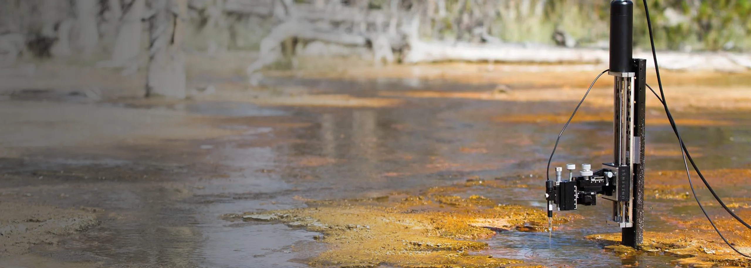
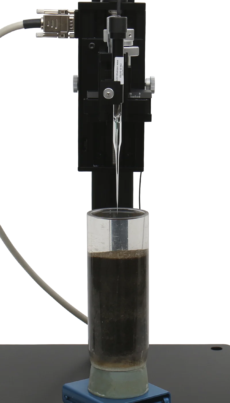
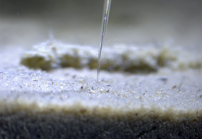
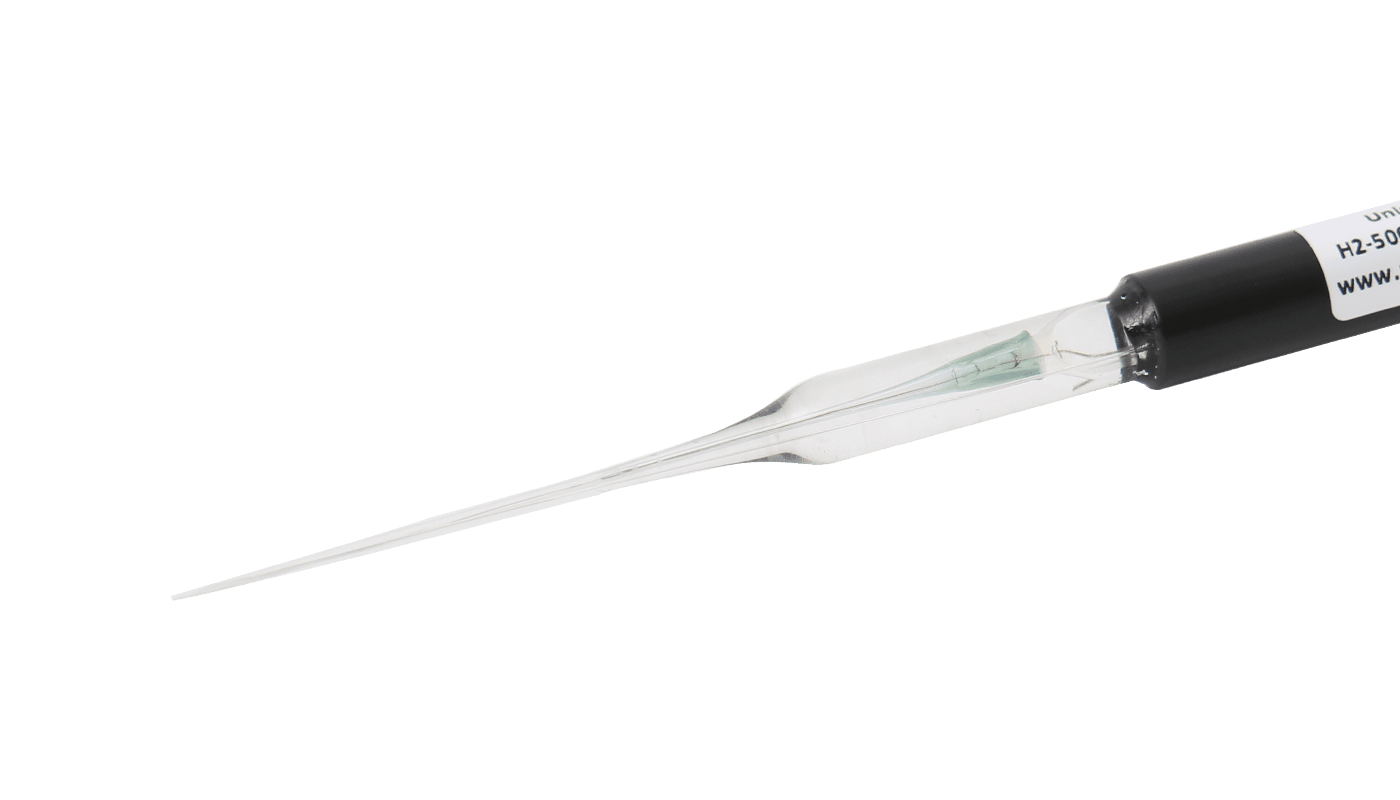
We flushed the water with air using an aquarium pump and a bubble stone to ensure a good circulation and to establish a well-defined Diffusive Boundary Layer (DBL) just above the sediment-water interface (figure 2 and 3). We made the oxygen microprofiles using a motorized MicroProfiling System and an oxygen microsensor with a tip size of 50 μm (OX-50).
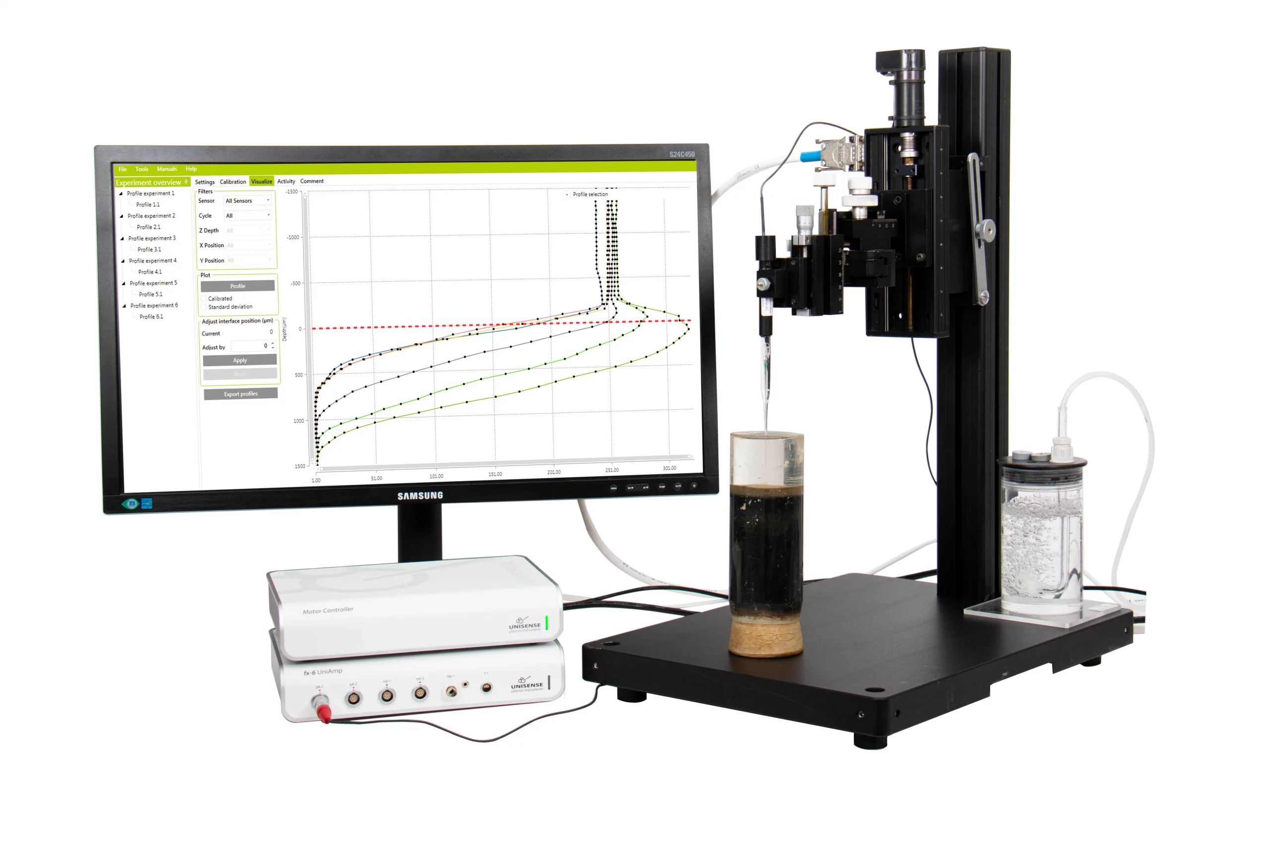
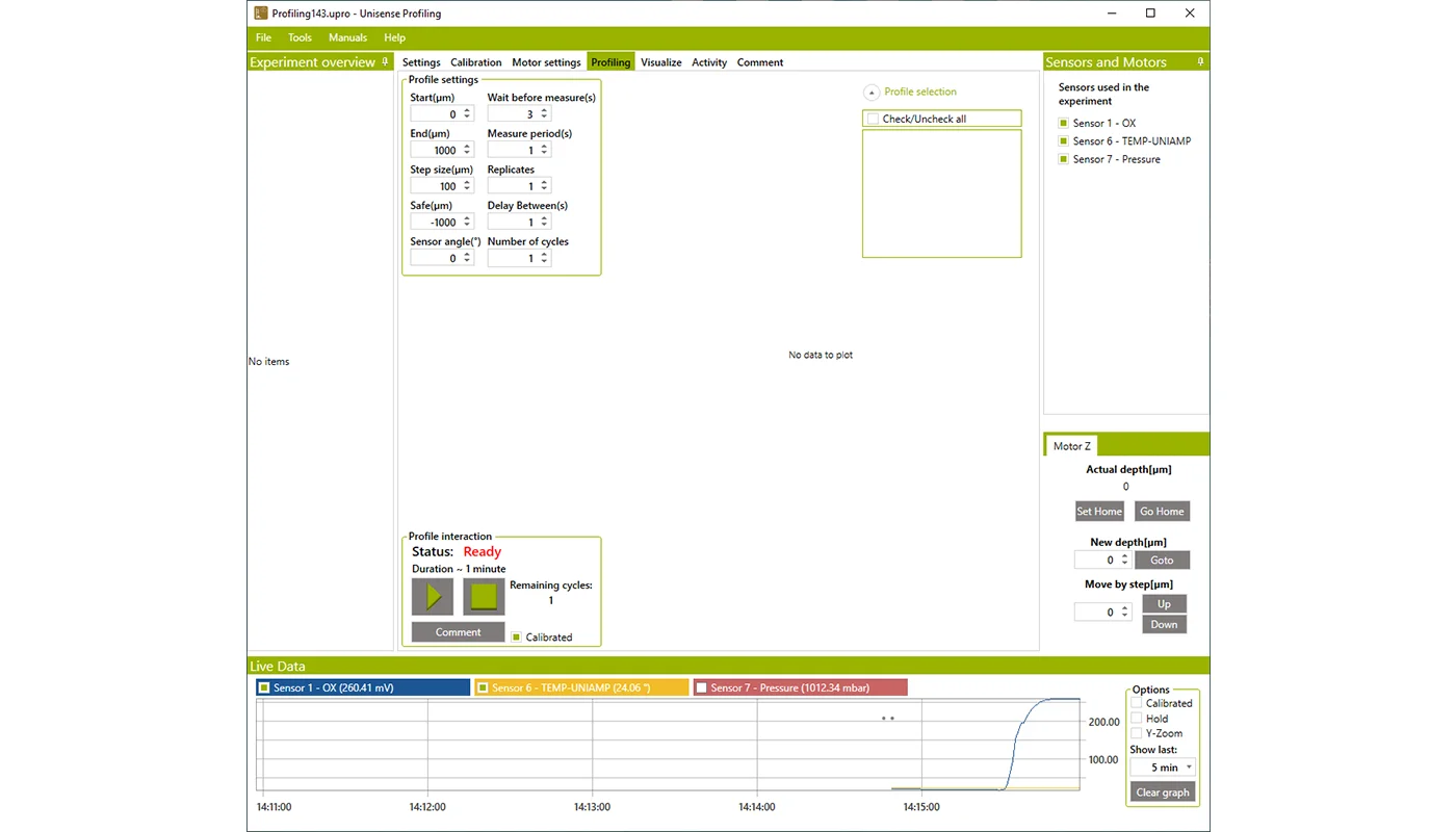
We used uSense Profile for sensor calibration, motor control and data collection. The oxygen concentration was measured in units of μmol/L. Data was collected with 50 μm step size, 3 seconds wait and 1 second measuring time.
Assumptions
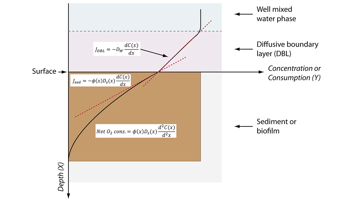
The software uses a one-dimensional mass conservation equation (Boudreau, 1984) for the rate calculations. The model assumes steady-state conditions where transport of oxygen occurs by diffusion, and it neglects effects of e.g. burial, groundwater flow, and wave actions. Temperature and salinity should be stable – preferably similar to the in-situ conditions. Click the image to read the description.
Sediment Water Interface
You can adjust the 0-line of the profile in the Visualization window of uSense Profile. The water - sediment is typically set to 0 μm depth. You can then use the profile with the adjusted 0-line in the Activity window.
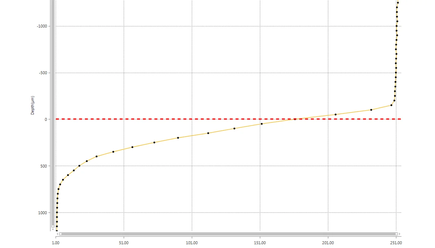
The interface – 0 μm depth – can sometimes be found from the oxygen profile, because the oxygen diffusion in water (D0) is typically higher than the oxygen diffusion in the sediment (Ds), which shows as a change in the slope at the water – sediment interface. The sediment surface is at the bottom of the DBL, where the oxygen profile changes direction.
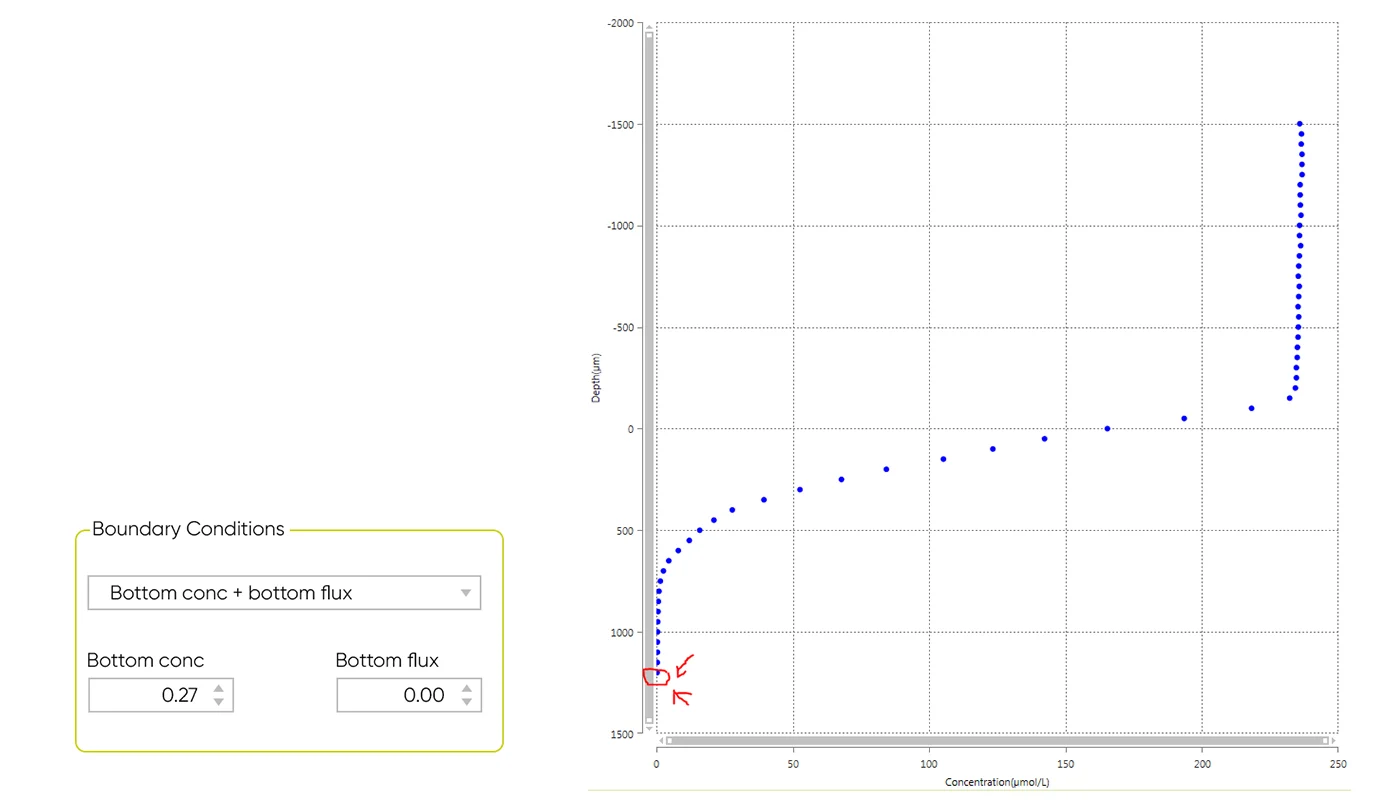
Boundary conditions: To constrain the model, two independent boundary values are needed for the analysis. In the program, you can select between 5 different pairs of boundary conditions, e.g. for oxygen profiles where the end concentration and flux deepest in the profile typically are 0 (as in the examples used here), the boundary condition ‘Bottom conc + bottom flux’ is typically used (Figure 4).
In the sediment from Limfjorden, we start with ‘Bottom conc + bottom flux’ boundary condition with the values at 0.27 μM for Bottom concentration and 0 for Bottom flux.
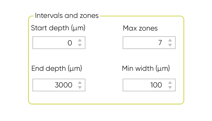
Interval and zones: Here you define the area of the profile you want to model. It is most appropriate to calculate rates in the depth interval where a consumption or production of oxygen takes place. In the model sediments, we start at the water - sediment interface (0 μm) and end where all oxygen is consumed at the bottom of the profile.
Max zones refers to how many volume-specific rate calculations the model should list (maximum 10 zones). The volume-specific rate is calculated from the profile using Fick’s second law of diffusion based on two or more measuring points. The appropriate number of zones can be estimated from the shape of the profile. Start by selecting a high number of zones e.g. 7. After the Analysis, the model highlights the most favorable number of zones based on the statistical values, SSE and p-value.
The minimum width of the zones should be at least twice the resolution of the profile. In our model profile, the resolution was 50 μm, so the minimum width should be at least 100 μm.
Diffusion Rate of Oxygen
In the Ds and Theta window of uSense Profile, the diffusion rates of oxygen in water (D0) and sediment (Ds) are defined. D0 is given in the oxygen diffusion table and is dependent on salinity and temperature. Enter the same temperature and salinity as measured when you made the profile.
Ds is dependent on D0 and porosity of the sediment (ϕ). The software lists three emperical formulas found in the literature, for the Ds calculations. The formula Ds = D0 × ϕ is often used in sediment with a high porosity – like a biofilm, microbial mat and soft silty sediments. The formula Ds = D0 × ϕ2 is typically used in sediments with lower porosity like sandy/silty sediment and compact mud. The formula Ds = D0/(1+3 × (1 - ϕ)) has been used in all kinds of sediments. You can also manually add your own Ds value.
In the sediment from Limfjorden the overlying water had a bottom temperature of 20 °C and a salinity of 15 ‰ which gives a D0 of 2.038 10-5 cm2 s-1. Ds is calculated based on Ds = D0 × ϕ, because the sediment had a relative high porosity, of 0.8, giving a Ds of 1.63 10-5 cm2 s-1.
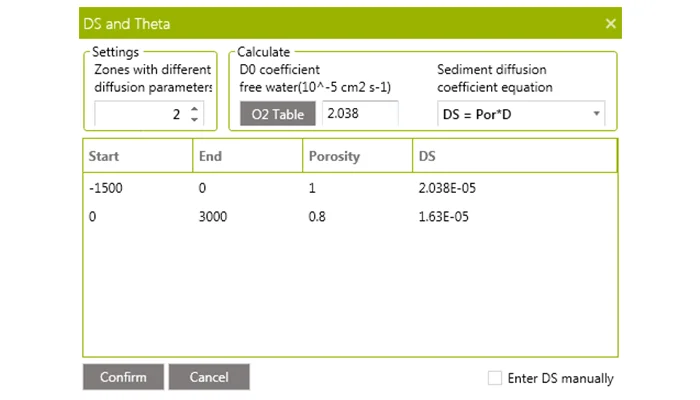
Porosity: The ratio between the volume of void space (like water) and the total volume of your sample. The porosity of the sediment is often determined as water content. If the porosity varies with depth, increase the number of zones and define the diffusion conditions for each depth interval. In the sediment from Limfjorden, we define Ds in two zones; one in the water column where Ds = D0 = 2.038 10-5 cm2 s-1 and one in the sediment where Ds = 1.63 10-5 cm-2 s-1.
Results
The results of the model calculation are listed in the Statistics table and the Profile figure.
When you receive the results from the model, it is important to verify if the results are scientifically correct. Below we will give you some factors you should give special attention to:
- The yellow modeled profile
- The volume based rate calculations
- Zone number and statistics
- Integrated production and consumption rates
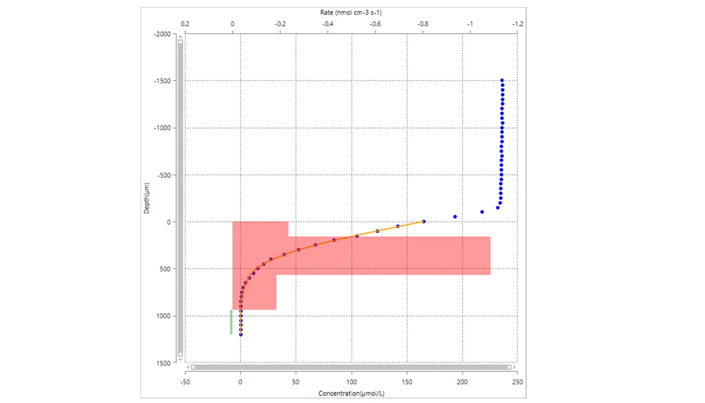
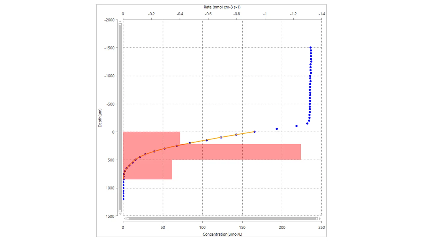
A model is good, if the yellow modeled profile is placed on top of the measured values at all depths. The green and red bars show the volume specific rate in the different depth zones.
Statistics after 1st analysis
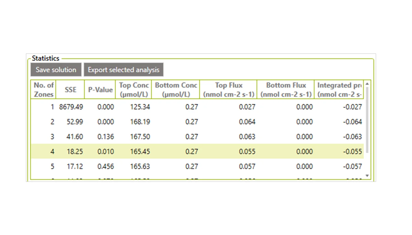
In the statistics table (figure 10), the model highlights the row with the optimal number of zones based on the statistics. The SSE indicates how well the measured and modeled profiles fit - the lower the SSE value the better. The P-Value may be used for selection of the best number of zones. The P-Value for n zones indicates whether increasing the number of zones from n - 1 to n resulted in a significantly improved fit.
Often P < 0.05 is used as the criterion. In Figure 10, going from 3 to 4 zones gave a significantly better fit (P = 0.010), whereas going from 4 to 5 zones did not (P = 0.456). In the table you also find the calculated oxygen flux and the integrated oxygen consumption or production rates.
In our model system, 4 zones provides the best statistical values and an integrated oxygen consumption rate of 0.055 nmol cm-2 s-1.
However, from the figure, we can see that the integrated rate was based on an oxygen production rate at the bottom of the profile, which scientifically is very unlikely and due to variation in data. To avoid this, we changed the depth interval to maximum depth of 850 μm. At 850 μm, the bottom oxygen concentration is 0.70 μM, which is used as the boundary conditions under ‘Bottom concentration’.
Statistics after 2nd analysis
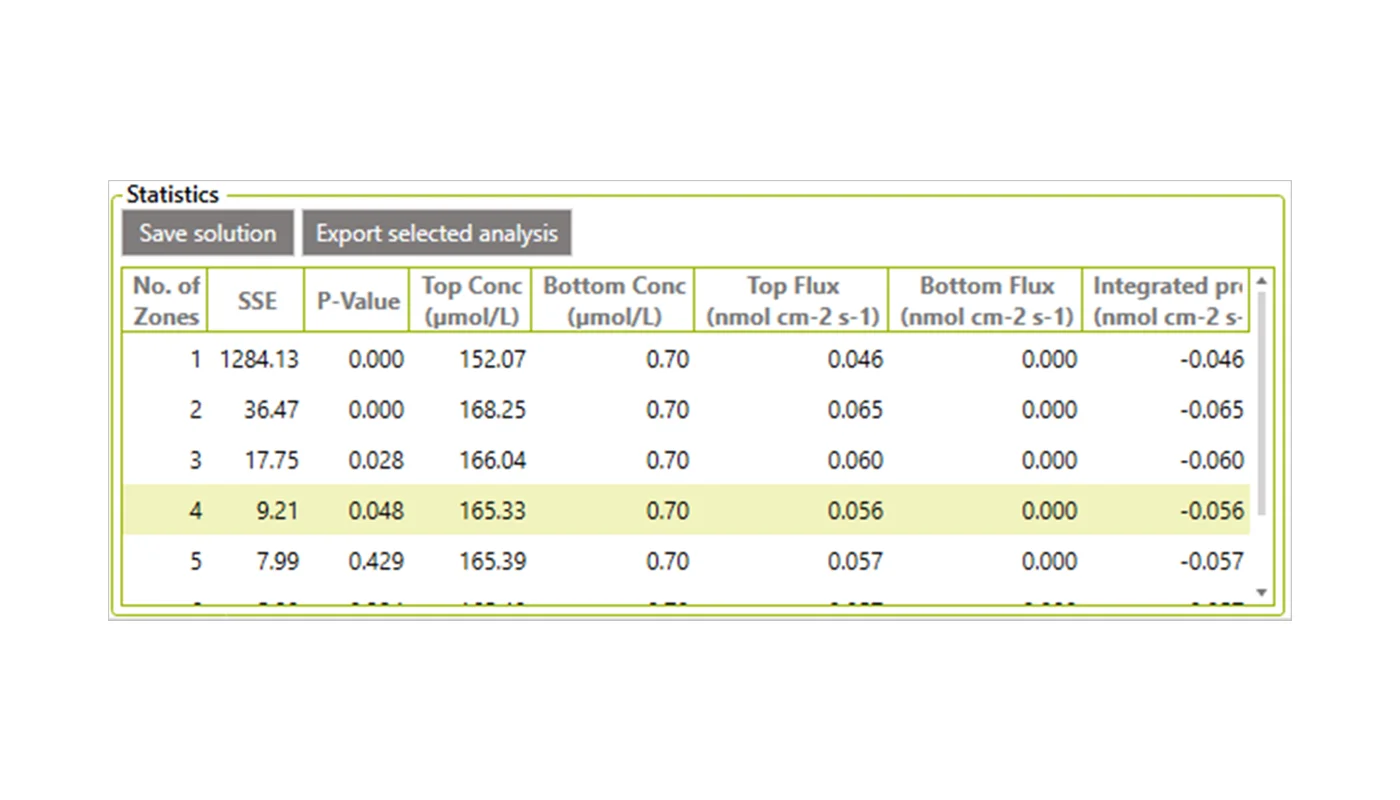
Running Analyze with these new parameters gave the result you can see in this image (click to enlarge).
Again the model suggests that 4 intervals result in the best solution (Figure 11). This provides an integrated oxygen consumption rate of 0.056 nmol cm-2 s-1. The SSE value is lower than in the first analysis, whereas the P-value is a bit higher.
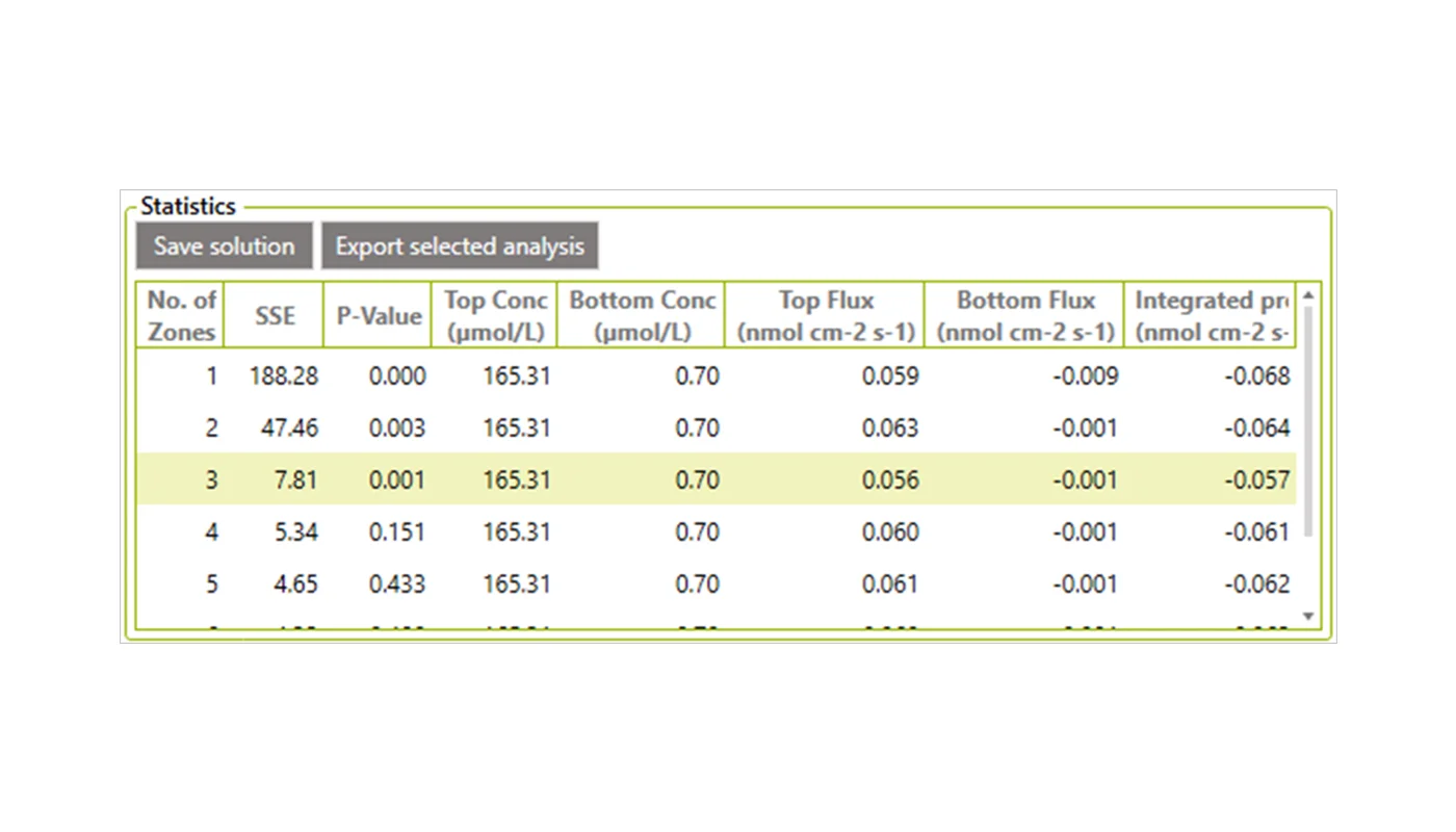
Statistics after 3rd analysis
In an attempt to improve the fit, we changed the boundary conditions, because at a depth of 850 μm there is still oxygen and a small oxygen flux is expected in the sediment. Therefore, we changed the boundary conditions from ‘Bottom conc + bottom flux’ to ‘Top conc + bottom conc’ and made a third analysis. The result gave an optimal zone number of 3 and an integrated oxygen consumption rate of 0.056 nmol cm-2 s-1 (Figure 12 and 13). The statistical values were now better than the previous solutions with an SSE value of 7.81 and a P-value of 0.001.
After trying to change other parameters (see also ‘Play around’ below), we decided to use the data from the 3rd analysis as our final result. We recommend to make similar calculations for minimum two more profiles from the same location.
Play Around
The quality of the model depends on the input data. Some input data are associated with relatively high uncertainty – e.g. the porosity. In order to get a feel for how sensitive the fit and the calculated rates are to the input data, we recommend to play around with the different input information - e.g.:
- Boundary conditions
- Depth interval
- The oxygen diffusion rate - e.g. by changing the temperature and salinity
- Change the formula for the Ds calculation
- Porosity
In our model a change of 2-3 °C or 2-3 ‰ in the calculation of D0 did not give an important change in our results, and neither did a change in the formula from Ds = D0 × ϕ to Ds = D0 x ϕ2 or changing the porosity from 0.8 to 0.85.
Final result
Using the uSense Profile software on a high-resolution oxygen profile made in an organic rich sediment core from Limfjorden in Denmark, we found that the oxygen penetration was approximately 950 μm and the integrated oxygen consumption rate was 0.057 nmol cm-2 s-1. The highest specific oxygen consumption rate, 1.25 nmol cm-3 s-1, was found at approx. 200 μm to 500 μm sediment depth.
These oxygen consumption rates are similar to the rate found in similar organic rich sediments (e.g. Glud 2008, Epping et al 1999).
Other solutes
The consumption and production rate of solutes like H2S, H2, and N2O can also be calculated in uSense Profile from high resolution profiles.
The general procedure for other solutes is the same as for oxygen, although the inputs may vary depending on the profile. For example, the sulfide concentration is often 0 at the surface of the sediment and high at the bottom, therefore the boundary condition ‘top conc and top flux’ of 0 is often used. The Diffusion coefficient (D0) for other gasses than oxygen can be calculated from the oxygen table “Seawater and Gases Table” by multiplying the table values with a constant specific for the different solutes: for H2S multiply by 0.7573, for H2 with 1.9470, and for N2O with 1.0049 (for more information see “Seawater and Gases Table”).
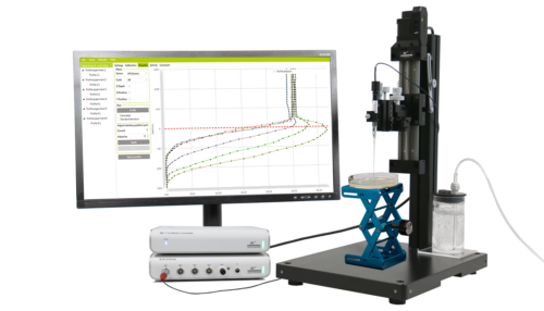
Microprofiles with extreme accuracy, high spatial and temporal resolution
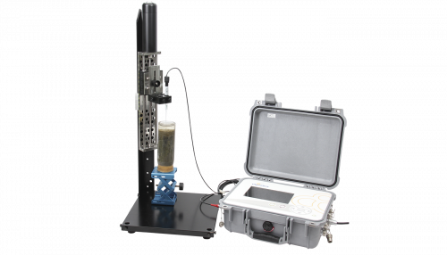
Water resistant Field MicroProfiling System to generate, study, and analyze microprofiles
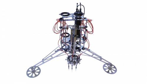
Complete system for shallow water microprofiling studies with 4 or 8 channels

Automated or manual profiling, data visualization, and activity rate calculations.